Create a dividend income tracker with Google Sheets by simply using pivot tables
As my investment strategy is to buy stocks that pay regular and stable dividends during a long-term period, I need to monitor my dividends income by stocks, by months, and by years, so that I can answer quickly and exactly the following questions:
- How much dividend did I receive on a given month and a given year?
- How much dividend did I receive for a given stock in a given year?
- Have a given stock's annual dividend per share kept increasing gradually over years?
- Have a given stock's annual dividend yield been stable over years?
In this post, I explain how to create a dividend tracker for a stock investment portfolio with Google Sheets by simply using pivot tables.

Table of Contents
Manage stock transactions with Google Sheets
I use a spreadsheet on Google Sheets to keep track of my stock portfolio's transactions. I insert a new transaction into the spreadsheet whenever I deposit money, withdraw money, use deposited money to buy stocks, receive money by selling stocks, and receive dividends by holding stocks. Each transaction is a row containing information about Date, Type, Symbol, Amount and Shares of that transaction. For further details, you should read my post Manage stock transactions with Google Sheets.

Create dividend tracker with Google Sheets
My questions in the introduction can be answered by finding relationships in terms of dividends between months and years or between stocks and years. In the same time, a pivot table helps to see relationships between data points in a spreadsheet. Therefore a dividend tracker here is a combination of several pivot tables originated from the Transactions sheet.
Track annual dividend amount of stocks
Here are the steps to create a pivot table to track annual dividend amount of stocks:
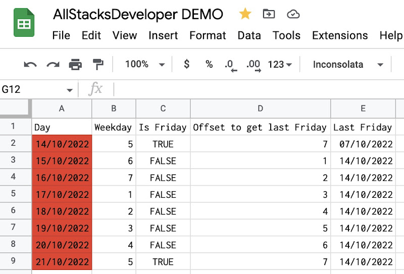
- As a preparation step, I create a support column (Year) for the year of each transaction. Year is derived from the Date column with this function:
=YEAR(A2) - To create a pivot table fom the transactions, I follow the steps below:
- Select all used columns in the Transactions sheet.
- In the menu at the top, click Insert and then Pivot table.
- Select the newly created pivot table sheet, if it’s not already open.
- As I want to know the annual dividend amount contributed by a given stock, I need to configure a pivot table as follow:
- In the Rows section, I click Add and select Symbol from the dropdown list.
- All symbols that appeared in transactions will be displayed as rows in the pivot table.
- I keep checked the Show totals check box because I want to know the total dividend contributed by a given stock since the beginning.
- In the Columns section, I click Add and select Year from the dropdown list.
- All years that appeared in transactions will be displayed as columns in the pivot table.
- I keep checked the Show totals check box because I want to know the total dividend contributed by all stocks on a given year.
- In the Values section, click Add, select Amount from the dropdown list, and choose Sum in the Summarize by select box.
- In the Filters section, I choose to filter by Type of transactions and select only DIVIDEND value in the dropdown list.
- In the Rows section, I click Add and select Symbol from the dropdown list.

As a result, I have a table with columns being years (sorted ascending), rows being stocks, and cells being the dividend amounts. I can quickly know the dividend amount contributed by any stock on any year by simply locating the corresponding cell in the table. In short, the pivot table gives me an overview picture of how much dividend each stock has contributed in each year and helps me to compare their performance.

Note: In fact, with all transactions tracked, it is not difficult to compute the amount of dividend contributed by a given stock on a given year, without using a pivot table.
For example, to know the amount of dividends contributed by the stock EPA:CS during the year 2020, I just simply need to sum the column Amount of all transactions, where:
- TYPE is DIVIDEND
- SYMBOL is EPA:CS
- DATE is after 31/12/2019
- DATE is before 01/01/2021
I can use the built-in SUMIFS function:
=SUMIFS(Transactions!D:D,Transactions!B:B,"DIVIDEND",Transactions!C:C,"EPA:CS",Transactions!A:A,">12/31/2019",Transactions!A:A,"<01/01/2021")
However, I need to repeat that formula if I want to query for another symbol or another year. Moreover, this way doesn't give me an overview picture of the dividends contribution among all stocks over years, as does a pivot table.
Track dividend amount by month and by year
To track dividend amount by month and by year, I just need to do another pivot table based on the same approach.
- As a preparation step, I create a support column (Month) for the month of each transaction. Month is derived from the Date column with this function:
=MONTH(A2) - I follow the same steps to create a pivot table from the transactions, and then configure it:
- In the Rows section, I add Month as rows and sort them ascending. I keep checked the Show totals check box because I want to know the total dividend collected on a given month over all years.
- In the Columns section, I add Year as columns and sort them ascending. I keep checked the Show totals check box because I want to know the total dividend collected in a given year.
- In the Values section, I add Amount and choose Sum in the Summarize by select box.
- In the Filters section, I choose to filter by Type of transactions and select only DIVIDEND value in the dropdown list.

As a result, I have a table with columns being years (sorted ascending), rows being months (sorted ascending), and cells being the dividend amounts. I can quickly know the dividend amount collected in any month of any year by simply locating the corresponding cell in the table. In short, the pivot table gives me an overview picture of how regularly and stably I have collected dividends.

Track annual dividend per share of stocks
Because each transaction is registered with the Amount and the number of Shares, it is easy to calculate the dividend per share on each transaction. To know the annual dividend per share of a stock, I can simply sum dividend per share of all transactions for that stock on a year.
To track the annual dividend per share of stocks, I just need to do another pivot table based on the same approach.
- As a preparation step, I create a support column (Transaction Unit) for amount by share of each transaction. The column is derived from the Amount column and the Shares column with this function:
=IF(ISBLANK(E2),,D2/E2) - I follow the same steps to create a pivot table from the transactions:
- In the Rows section, I add Symbol as rows.
- In the Columns section, I add Year as columns and sort them ascending.
- In the Values section, I add Transaction Unit and choose Sum in the Summarize by select box.
- In the Filters section, I choose to filter by Type of transactions and select only DIVIDEND value in the dropdown list.
As a result, I have a table with columns being years (sorted ascending), rows being stocks, and cells being the annual dividend per share. If I hold shares of a company long enough, the table allows me to track how the annual dividend per share of my holding stocks evolve over time.

Note: On the table, the dividend per share might not be the actual dividend per share of a stock in a given year. For example, in 2019, a company distributed dividends every quarter and I hold its shares for only 3 quarters, I would receive only 3 dividend payments. As a result, the tracker takes only into account those 3 dividend payments while calculating the dividend per share for that stock in 2019.
Track annual dividend yield of stocks
The annual dividend yield is a result of dividing the annual dividend per share by the price per share. As the annual dividend per share is already computed in the previous section, to compute the annual dividend yield, I still need to identify the price per share. However, during a year, a stock has many price points, and which one should be used among the price on the last day of year, the average price during a year, etc.? As an investor who keep track carefully transactions for a stock, I can easily know the cost per share of a stock in my portfolio. Therefore, I use the cost per share as a reference price to compute the dividend yield.
The cost per share of a stock in my portfolio is a result of dividing its cost by the number of shares that I have for that stock.
- The cost is the sum of Amount for all BUY an SELL transactions related to that stock.
- The number of shares is the sum of Shares for all BUY and SELL transactions related to that stock.
For example, to compute the unit cost for the EPA:CS stock until 01/01/2021, I need to compute how much money I have invested in that stock in exchange for how many shares (until 01/01/2021). It is not a difficult task by using SUMIFS function of Google Sheets:
Sum all Amount of BUY, SELL transactions for the EPA:CS stock until 01/01/2021
=ABS((SUMIFS(D:D,C:C,"EPA:CS",A:A,"<=01/01/2021",B:B,"BUY") +
SUMIFS(D:D,C:C,"EPA:CS",A:A,"<=01/01/2021",B:B,"SELL")))

Sum all Shares of BUY, SELL transactions for the EPA:CS stock until 01/01/2021
=(SUMIFS(E:E,C:C,"EPA:CS",A:A,"<=01/01/2021",B:B,"BUY") +
SUMIFS(E:E,C:C,"EPA:CS",A:A,"<=01/01/2021",B:B,"SELL"))

The unit cost for the EPA:CS stock on 01/01/2021 is:
=ABS((SUMIFS(D:D,C:C,"EPA:CS",A:A,"<=01/01/2021",B:B,"BUY") + SUMIFS(D:D,C:C,"EPA:CS",A:A,"<=01/01/2021",B:B,"SELL"))) /
(SUMIFS(E:E,C:C,"EPA:CS",A:A,"<=01/01/2021",B:B,"BUY") + SUMIFS(E:E,C:C,"EPA:CS",A:A,"<=01/01/2021",B:B,"SELL"))
To track the annual dividend yield of stocks, I just need to do another pivot table based on the same approach.
- As a preparation step, I create 4 support columns in the Transactions sheet:
- Cost After A Transaction: is the cost for the stock presented in the transaction, taken into account the transaction's impact
- Shares After A Transaction: is the number of shares for the stock presented in the transaction, taken into account the transaction's impact
- Unit Cost After A Transaction: is the unit cost for the stock presented in the transaction, taken into account the transaction's impact
- Dividend Yield Based On Unit Cost: is the transaction unit divided by the unit cost in case of a DIVIDEND transaction, taken into account the transaction's impact
Cost After A Transaction on the cell I2:
=IF(ISBLANK(C2),"",ABS((SUMIFS(D:D,C:C,C2,A:A,"<="&A2,B:B,"BUY") + SUMIFS(D:D,C:C,C2,A:A,"<="&A2,B:B,"SELL"))))

Shares After A Transaction on the cell J2:
=IF(ISBLANK(C2),,(SUMIFS(E:E,C:C,C2,A:A,"<="&A2,B:B,"BUY") + SUMIFS(E:E,C:C,C2,A:A,"<="&A2,B:B,"SELL")))

Unit Cost After A Transaction on the cell K2:
=IF(J2>0,I2/J2,"")

Dividend Yield Based On Unit Cost on the cell L2:
=IF(B2="DIVIDEND",H2/K2,"")
- I follow the same steps to create a pivot table from the transactions:
- In the Rows section, I add Symbol as rows.
- In the Columns section, I add Year as columns and sort them ascending.
- In the Values section, I add Dividend Yield Based On Unit Cost and choose Sum in the Summarize by select box.
- In the Filters section, I choose to filter by Type of transactions and select only DIVIDEND value in the dropdown list.
As a result, I have a table with columns being years (sorted ascending), rows being stocks, and cells being the approximate annual dividend yield. The important thing is that those dividend yields are calculated based on my actual cost per share for those stocks in my portfolio. In short, the pivot table gives me an insightful picture to compare the performance in terms of annual dividend yield among my holding stocks.

Note: The annual dividend yield calculated by this way must be understood with cautious, because it is the sum of all dividend yields during one year. For example, if a stock pays dividend several times a year and in the same time, its unit cost fluctuates greatly during that one year, the sum of dividend yields might be abnormal.
Demo
Demo spreadsheet: sample dividend tracker with Google Sheets
The sample dividend tracker spreadsheet includes:
- Transactions sheet stores all transactions of the sample portfolio.
- Annual Dividend Amount sheet contains the pivot table showing dividend amount by stocks and by years.
- Dividend Amount By Month By Year sheet contains the pivot table showing dividend amount by months and by years.
- Annual Dividend Per Share sheet contains the pivot table showing annual dividend per share of stocks.
- Annual Dividend Yield sheet contains the pivot table showing annual dividend yield of stocks.
- Annual Dividend Amount, Dividend Per Share, Yield sheet contains the pivot table showing annual dividend amount, annual dividend per share, annual dividend yield of stocks.
Conclusion
In this post, I have explained step-by-step how to create a dividend tracker with Google Sheets. The process involves registering a portfolio's transactions in a spreadsheet and then creating pivot tables based on those transactions. The dividend tracker gives me an overview picture of my dividend income and helps me adjust my decisions to make my investment strategy always on track.
References
- Manage stock transactions with Google Sheets
- Create & use pivot tables on Google Sheets
- Create and edit pivot tables on Google Sheets
- SUMIFS function on Google Sheets
- Use conditional formatting rules in Google Sheets
Disclaimer
The post is only for informational purposes and not for trading purposes or financial advice.
Feedback
If you have any feedback, question, or request please:
- leave a comment in the comment section
- write me an email to allstacksdeveloper@gmail.com
Support this blog
If you value my work, please support me with as little as a cup of coffee! I appreciate it. Thank you!

Share with your friends
If you read it this far, I hope you have enjoyed the content of this post. If you like it, share it with your friends!


Comments
Post a Comment