GOOGLEFINANCE Best Practices
Anyone using Google Sheets to manage stock portfolio investment must know how to use the GOOGLEFINANCE function to fetch historical prices of stocks. As I have used it extensively to manage my stock portfolio investment in Google Sheets, I have learned several best practices for using the GOOGLEFINANCE function that I would like to share in this post.

Table of Contents
- Some inconveniences of using the GOOGLEFINANCE function to fetch historical prices
- Include today price in the historical prices returned by the GOOGLEFINANCE function
- Ignore the Date column returned by the GOOGLEFINANCE function
- Ignore the headers row returned by the GOOGLEFINANCE function
- Keep only the price
- Create a dedicated sheet to store prices for each stock to limit calls to GOOGLEFINANCE function
- Use QUERY function instead of VLOOKUP function for looking up by date
- Conclusion
- Disclaimer
- Feedback
- Support this blog
- Share with your friends
Some inconveniences of using the GOOGLEFINANCE function to fetch historical prices
In Google Sheets, the GOOGLEFINANCE function allows fetching historical prices of stocks. GOOGLEFINANCE("NASDAQ:TSLA","price",TODAY()-30,TODAY()) returns the prices of tesla stock during the last 30 days. The returned results are a table of two columns with headers: Date and Close. The table is automatically sorted in ascending order by date. However, I have identified some inconveniences of using the GOOGLEFINANCE function to fetch historical prices:
- The stock's latest price is not included in the price. If today is 29/09/2022, the results include only prices until 28/09/2022 as shown in the below picture.
- In many scenarios, I need to use only the prices as a parameter to another formula but it is not quite practical because of the presence of the headers row and the Date column.
- The Date column including time causes some difficulties in comparing dates, especially, in the case of using VLOOKUP.
- The abusive use of the GOOGLEFINANCE can cause performance issue for the spreadsheet.

Include today price in the historical prices returned by the GOOGLEFINANCE function
The GOOGLEFINANCE function returns the historic prices of stocks in the form of a table having two columns and a headers row. In Google Sheets, a table is a two-dimensional array and the brackets { } syntax is used for working with the arrays. As the table is sorted in ascending order by date, including today's price requires simply adding a new row at the end. The new row consists of today's date and today's price.
={GOOGLEFINANCE("NASDAQ:TSLA","price",TODAY()-7,TODAY());{TODAY(),GOOGLEFINANCE("NASDAQ:TSLA")}}
- To create a new row, I use { } with a comma
- To add a new row to an existing table, I use { } with a semicolon

Ignore the Date column returned by the GOOGLEFINANCE function
I use the INDEX function on the results returned by GOOGLEFINANCE to ignore the Date column.
=INDEX(GOOGLEFINANCE("NASDAQ:TSLA","price",TODAY()-7,TODAY()),0,2)

Ignore the headers row returned by the GOOGLEFINANCE function
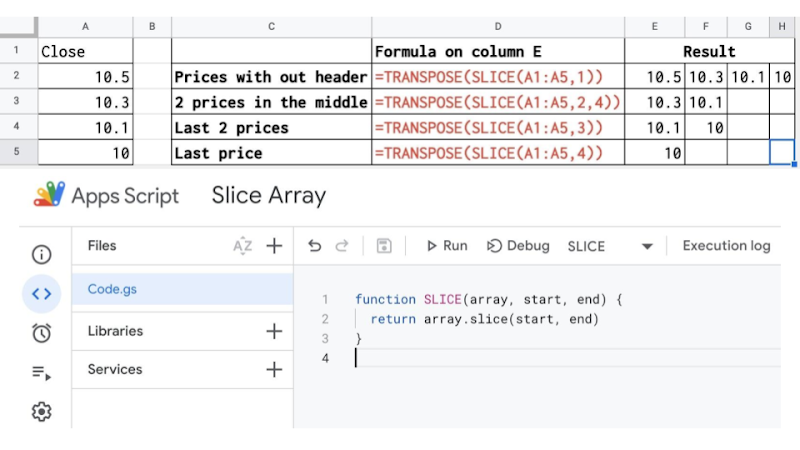
It is more complicated to remove the header row than the Date column. The results are a two-dimensional array indexed by row, then by column. Removing the header row is like removing the first element of an array. As far as I have searched, I have not found any built-in formula to remove the first element of an array in Google Sheets. However, it is really simple to remove an element from an array with JavaScript, and Google Sheets supports the customizations with Google Apps Script that is based on JavaScript. That means I create a custom function with Google Apps Script and then use it inside Google Sheets. I explained the details in the post Slice array in Google Sheets. The below formula is how I apply it:
=SLICE(GOOGLEFINANCE("NASDAQ:TSLA","price",TODAY()-7,TODAY()),1)

Keep only the price
It is the combination of ignoring the Date column and the header row from data returned by the GOOGLEFINANCE function.
=SLICE(INDEX(GOOGLEFINANCE("NASDAQ:TSLA","price",TODAY()-7,TODAY()),0,2),1)
Create a dedicated sheet to store prices for each stock to limit calls to GOOGLEFINANCE function
Too many calls to the GOOGLEFINANCE function to get historical prices can cause performance issues for the spreadsheet. It is a redundant task if it is for the same stock and the same duration. To avoid that, I create a dedicated sheet for each stock, then call GOOGLFINANCE once to get its historical price. I then use other built-in functions in Google Sheets to look up that sheet to get prices if I need them at others locations.
For example:
- For the tesla stock, I create a sheet and name it NASDAQ:TSLA
- On the cell A1 of that sheet, I put the formula GOOGLEFINANCE("NASDAQ:TSLA","price",TODAY()-7,TODAY())
- When I need historical prices of tesla stock at other locations, I lookup for them in the NASDAQ:TSLA sheet instead of calling GOOGLFINANCE again.
Use QUERY function instead of VLOOKUP function for looking up by date
Because the Date column returned from GOOGLEFINANCE contains time data, it is difficult to use VLOOKUP for looking for a particular date. In Google Sheets, 9/28/2022 does not have the same numerical value as 9/28/2022 16:00:00, so VLOOKUP can not match them exactly. Instead, I use the QUERY function:
=QUERY(INDIRECT("NASDAQ:TSLA!A:B"),"select B where datediff(A, date '2022-09-26')=0 limit 1",0)
Another advantage of using the QUERY function over the VLOOKUP function is that the QUERY function can return multiple values whereas VLOOKUP returns only a single value.
=QUERY(INDIRECT("NASDAQ:TSLA!A:B"),"select B where A < date '2022-09-26' and A > date '2022-09-01' order by A asc",0)
Conclusion
In this post, I shared several best practices for using the GOOGLEFINANCE function that I have learned along the way of using Google Sheets to manage my stock portfolio investment. I will update this post whenever I learn an interesting practice. If you have any best practices for using Google Sheets, please share them in the comment section!
This post is part of a series of posts about effectively using the SPARKLINE function and the GOOGLEFINANCE function for managing a stock investment in Google Sheets.


Disclaimer
The post is only for informational purposes and not for trading purposes or financial advice.
Feedback
If you have any feedback, question, or request please:
- leave a comment in the comment section
- write me an email to allstacksdeveloper@gmail.com
Support this blog
If you value my work, please support me with as little as a cup of coffee! I appreciate it. Thank you!

Share with your friends
If you read it this far, I hope you have enjoyed the content of this post. If you like it, share it with your friends!

Comments
Post a Comment