
Slice array in Google Sheets

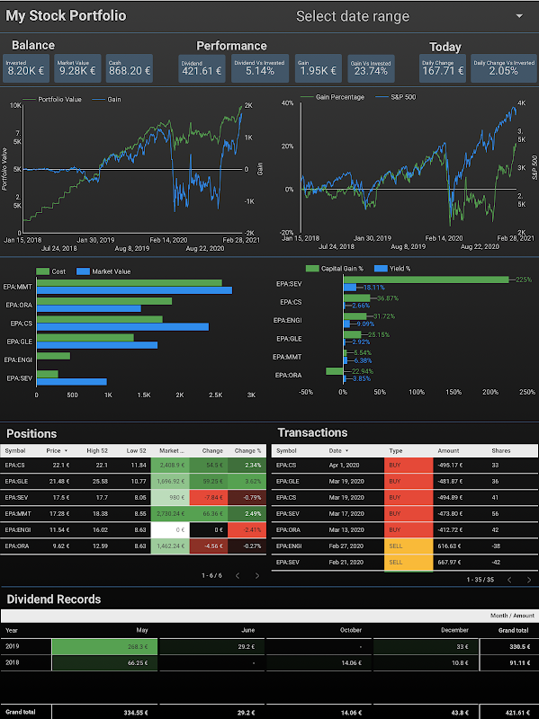
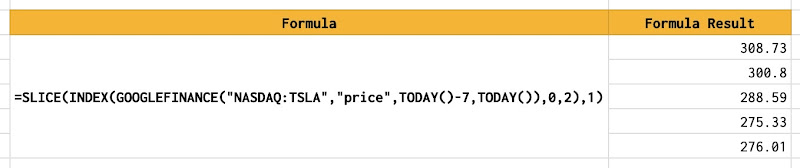
Many functions in Google Sheets return an array as the result. However, I find that there is a lack of built-in support functions in Google Sheets when working with an array. For example, the GOOGLEFINANCE function can return the historical prices of a stock as a table of two columns and the first-row being headers Date and Close. How can I ignore the headers or remove the headers from the results?

Slice array in Google Sheets

Make any JavaScript method available in Google Sheets

In JavaScript, there is the SLICE method that can return a part of an array. If I have an array const pricesWithHeader = ['Close', 10.5, 10.3, 10.1, 10.0];, to get only the last 4 elements [10.5, 10.3, 10.1, 10.0], I can apply the SLICE method like const pricesWithoutHeader = pricesWithHeader.slice(1);. How to slice an array in Google Sheets?

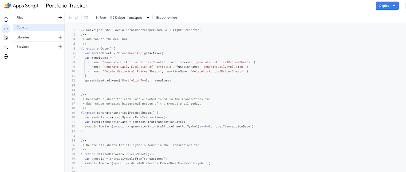
Google Sheets has scripting capability with Apps Script based on JavaScript. So to slice an array in Google Sheets, I need to create a SLICE method in Apps Script that wraps the original SLICE method of JavaScript. By doing so, the SLICE function is available to use in every cell of a spreadsheet.

Demo and source code

Demo spreadsheet: How to slice array in Google Sheets

References

Disclaimer

The post is only for informational purposes and not for trading purposes or financial advice.

Feedback

If you have any feedback, question, or request please:

Support this blog

If you value my work, please support me with as little as a cup of coffee! I appreciate it. Thank you!

Share with your friends

If you read it this far, I hope you have enjoyed the content of this post. If you like it, share it with your friends!

Comments

  1. Here's a Google Sheets formula similar to JavaScript slice() to return a subset of rows from a range/array:
    =let(
    array,A74:A81,
    start,B72 +n("First row is 1, last row is -1"),
    end,B73 +n("Same row counting"),
    startv, if(start=0,1,start) +n("0 starts from the first row"),
    endv, if(end=0,-1,end) +n("0 ends at the last row"),
    rows,rows(array),
    offset,max(0,if(startv>=0,startv-1,rows+startv)),
    limit,max(0,if(endv>=0,endv-startv+1,rows+endv+1-offset)),
    q, query(array,"select * limit "&limit&" offset "&offset&" "),
    q
    )

    ReplyDelete
  2. It can be converted to a named function, then used like: =SLICE({1,2,3,4,5}, 2,-2)

    ReplyDelete

Post a Comment

Popular posts

Compute cost basis of stocks with FIFO method in Google Sheets

Compute cost basis of stocks with FIFO method in Google Sheets

After selling a portion of my holdings in a stock, the cost basis for the remain shares of that stock in my portfolio is not simply the sum of all transactions. When selling, I need to decide which shares I want to sell. One of the most common accounting methods is FIFO (first in, first out), meaning that the shares I bought earliest will be the shares I sell first. As you might already know, I use Google Sheets extensively to manage my stock portfolio investment, but, at the moment of writing this post, I find that Google Sheets does not provide a built-in formula for FIFO. Luckily, with lots of effort, I succeeded in building my own FIFO solution in Google Sheets, and I want to share it on this blog. In this post, I explain how to implement FIFO method in Google Sheets to compute cost basis in stocks investing.
Compute daily evolutions of a stock portfolio with Google Sheets and Apps Script

Compute daily evolutions of a stock portfolio with Google Sheets and Apps Script

When it comes to investment, it is not only important to know the up-to-date state of portfolio but also to track its evolution day by day. We need to know on a specific day, how much money has been invested in the portfolio, the current market value of owned shares, the available cash and the current profit. Visualizing those historical data points on a time-based graph helps us to identify which transactions were good and which were bad. This post shows how to compute automatically those historical data points by using data in Transactions sheet and the built-in GOOGLEFINANCE function of Google Sheets. A sample spreadsheet can be found in this post Demo stock portfolio tracker with Google Sheets . You can take a look at the sample spreadsheet to have an idea of how the data is organized and related. It is possible to make a copy of the spreadsheet to study it thoroughly.
GOOGLEFINANCE Best Practices

GOOGLEFINANCE Best Practices

Anyone using Google Sheets to manage stock portfolio investment must know how to use the GOOGLEFINANCE function to fetch historical prices of stocks. As I have used it extensively to manage my stock portfolio investment in Google Sheets , I have learned several best practices for using the GOOGLEFINANCE function that I would like to share in this post.
Create personal stock portfolio tracker with Google Sheets and Google Data Studio

Create personal stock portfolio tracker with Google Sheets and Google Data Studio

I have been investing in the stock market for a while. I was looking for a software tool that could help me better manage my portfolio, but, could not find one that satisfied my needs. One day, I discovered that the Google Sheets application has a built-in function called GOOGLEFINANCE which fetches current or historical prices of stocks into spreadsheets. So I thought it is totally possible to build my own personal portfolio tracker with Google Sheets. I can register my transactions in a sheet and use the pivot table, built-in functions such as GOOGLEFINANCE, and Apps Script to automate the computation for daily evolutions of my portfolio as well as the current position for each stock in my portfolio. I then drew some sort of charts within the spreadsheet to have some visual ideas of my portfolio. However, I quickly found it inconvenient to have the charts overlapped the table and to switch back and forth among sheets in the spreadsheet. That's when I came to know the existen...
Use SPARKLINE to create 52-week range price indicator chart for stocks in Google Sheets

Use SPARKLINE to create 52-week range price indicator chart for stocks in Google Sheets

The 52-week range price indicator chart shows the relative position of the current price compared to the 52-week low and the 52-week high price. It visualizes whether the current price is closer to the 52-week low or the 52-week high price. In this post, I explain how to create a 52-week range price indicator chart for stocks by using the SPARKLINE function and the GOOGLEFINANCE function in Google Sheets.
Compare stock investment portfolio to market indexes

Compare stock investment portfolio to market indexes

As investors, we always want to see our portfolio grows over time. If a portfolio made a 1000$ of gain in one year, is it good enough? Should we gauge the portfolio's performance against an alternative investment, for instance, a market index? Should we aim to beat that index? In this post, we will see how to compare a stock portfolio to market indexes by using Google Sheets, Apps Script, and Google Data Studio.
Stock Correlation Analysis With Google Sheets

Stock Correlation Analysis With Google Sheets

Correlation is a statistical relationship that measures how related the movement of one variable is compared to another variable. For example, stock prices fluctuate over time and are correlated accordingly or inversely to one another. Understanding stock correlation and being able to perform analysis are very helpful in managing a stock portfolio investment. In this post, I explain in details how to perform correlation analysis among stocks in Google Sheets.
Monitor stock investment portfolio with Pivot table and GOOGLEFINANCE function in Google Sheets

Monitor stock investment portfolio with Pivot table and GOOGLEFINANCE function in Google Sheets

As an investor, it is important to know the latest state of the stock portfolio. We need to know what stocks currently owned in the portfolio, how many shares for each one, how much dividend or gain contributed so far by each stock, etc. As we have registered stock transactions in a spreadsheet with Google Sheets, we can easily have the latest update from the stock portfolio by using pivot tables and GOOGLEFINANCE function.
Demo how to use XIRR and XNPV functions of Google Sheets to calculate internal rate of return (IRR) and net present value (NPV) for a stock portfolio

Demo how to use XIRR and XNPV functions of Google Sheets to calculate internal rate of return (IRR) and net present value (NPV) for a stock portfolio

I have explained the idea of using Google Sheets functions to calculate internal rate of return (IRR) and net present value (NPV) for a stock portfolio . The process consists mainly of three steps: Identify cash flows from transactions managed in a Google Sheets spreadsheet Choose a discount rate based on personal preferences Apply XIRR and XNPV functions of Google Sheets In this post, I demonstrate step-by-step how to apply this process to calculate internal rate of return (IRR) and net present value (NPV) for a stock portfolio at 3 levels.