Demo how to use XIRR and XNPV functions of Google Sheets to calculate internal rate of return (IRR) and net present value (NPV) for a stock portfolio
I have explained the idea of using Google Sheets functions to calculate internal rate of return (IRR) and net present value (NPV) for a stock portfolio. The process consists mainly of three steps:
- Identify cash flows from transactions managed in a Google Sheets spreadsheet
- Choose a discount rate based on personal preferences
- Apply XIRR and XNPV functions of Google Sheets
In this post, I demonstrate step-by-step how to apply this process to calculate internal rate of return (IRR) and net present value (NPV) for a stock portfolio at 3 levels.
 and net present value (NPV) for a stock investment portfolio")
Table of Contents
- Demo spreadsheet's structure
- Calculate internal rate of return (IRR) and net present value (NPV) for each stock in a portfolio
- Calculate internal rate of return (IRR) and net present value (NPV) for a group of stocks (by industry, by sector, by country, etc.) in a portfolio
- Calculate internal rate of return (IRR) and net present value (NPV) for a whole portfolio
- Make a copy
- Conclusion
- Series: how to calculate internal rate of return (IRR) and net present value (NPV) for a stock portfolio in Google Sheets
- Disclaimer
- Feedback
- Support this blog
- Share with your friends
Demo spreadsheet's structure
These guides are carried out on a spreadsheet that has a structure as below:
- The Transactions sheet contains the sample portfolio's transactions. A transaction has essentially information about date, type (BUY, SELL, DEPOSIT, WITHDRAW, and DIVIDEND), symbol of the involved stock, amount of money, and number of shares as defined in the post how to manage stock transactions with Google Sheets.
- The Companies sheet contains additional information about stocks presented in the sample portfolio, especially their industries and sectors.
- The Configuration sheet is where the discount rate is defined.
- The Values sheet is a pivot table from the Transactions sheet. It shows the latest state for each stock presented in the sample portfolio such as: Total Buy (Cost), Market Value, Gain, ROI, etc. The task is to calculate internal rate of return (IRR) and net present value (NPV) for each stock.
- The Industries sheet is a pivot table from the Values sheet. It shows the latest state for each industry presented in the sample portfolio such as: Total Buy (Cost), Market Value, Gain, ROI, etc. The task is to calculate internal rate of return (IRR) and net present value (NPV) for each industry.
- The Overview sheet shows the latest state for the whole portfolio such as: current portfolio value, current invested amount, current gain, etc. The task is to calculate internal rate of return (IRR) and net present value (NPV) for the sample portfolio.
As the discount rate is already defined in the Configuration, it leaves me only two steps to complete:
- Identify the cash flows by filtering the Transactions sheet
- Put the discount rate and the cash flows into the formulas XIRR and XNPV
Calculate internal rate of return (IRR) and net present value (NPV) for each stock in a portfolio
As cash flows for a stock in a portfolio are transactions of type BUY, SELL, and DIVIDEND related to that stock, to identify those cash flows, it is simply to filter the Transactions by the stock's symbol.
The function FILTER in Google Sheets allows to do that easily. To get all transactions of the stock EPA:ABCA, here is the formula:
=FILTER(Transactions!A:E,Transactions!C:C="EPA:ABCA")
Each transaction in the result contains respectively Date, Type, Symbol, Amount, and Shares.
For the XIRR formula, cash flows can be entered in any order but for the XNPV formula, cash flows must be ordered ascending by time. To keep it consistent, we should better sort them all ascending by time for both cases. To do that, I use the SORT function in Google Sheets:
=SORT(FILTER(Transactions!A:E,Transactions!C:C="EPA:ABCA"),1,true)

- Date is the first column in the range
- True for sorting ascending
As XIRR and XNPV functions demand cash flows amount and date separately, I use the INDEX function in Google Sheets to extract column from a range:
Because Date is the first column, therefore the formula for extracting the cash flows date is:

=INDEX(SORT(FILTER(Transactions!A:E,Transactions!C:C="EPA:ABCA"),1,true),,1)

Because Amount is the forth column, therefore the formula for extracting the cash flows amount is:

=INDEX(SORT(FILTER(Transactions!A:E,Transactions!C:C="EPA:ABCA"),1,true),,4)
With the cash flows identified for the stock EPA:ABCA, and the discount rate defined at Configuration!B2, here are the formulas to calculate internal rate of return (IRR) and net present value (NPV) for the stock EPA:ABCA:
=XIRR(
  INDEX(SORT(FILTER(Transactions!A:E,Transactions!C:C="EPA:ABCA"),1,true),,4),
  INDEX(SORT(FILTER(Transactions!A:E,Transactions!C:C="EPA:ABCA"),1,true),,1)
)

=XNPV(
  Configuration!B2,
  INDEX(SORT(FILTER(Transactions!A:E,Transactions!C:C="EPA:ABCA"),1,true),,4),
  INDEX(SORT(FILTER(Transactions!A:E,Transactions!C:C="EPA:ABCA"),1,true),,1)
)
For the stock EPA:ABCA, the internal rate of return (IRR) is 9.92% which is less than 10% targeted. On the other side, the net present value (NPV) is also a negative number -0.2498 for the same stock. The two indicators both mean my investment in EPA:ABCA don't give me the 10% annual rate I expected.
If you notice, EPA:ABCA is a stock that I don't have anymore in my portfolio. I sold out that stock. That means all cash flows for EPA:ABCA are presented as transactions. However, for stocks that I am still holding, the last cash flow is not yet presented in the Transactions sheet. That last cash flow is simply the amount I receive if I decided to sell my holding of the stock today, or in other word, the stock's current market value based on its latest price.
For example, EPA:ETL is a stock that I still own 479 shares in my portfolio. I can easily find its latest price with GOOGLEFINANCE function. From that, it is so simple to calculate the current market value of EPA:ETL in my portfolio. The tricky part is how to append that current market value into the list of cash flows filtered from the Transactions sheet. To append one element to a list of elements, I use the brackets {} syntax. For instance, ={A1:A10; 100} will add 100 to the list of elements presented from A1 to A10.
So here are the formulas to identify cash flows amount and date for EPA:ETL, a stock that is still hold in the portfolio:
={INDEX(SORT(FILTER(Transactions!A:E,Transactions!C:C="EPA:ETL"),1,true),,1);TODAY()}

={INDEX(SORT(FILTER(Transactions!A:E,Transactions!C:C="EPA:ETL"),1,true),,4);479*GOOGLEFINANCE("EPA:ETL")}
With the cash flows identified for the stock EPA:ETL, and the discount rate defined at Configuration!B2, here are the formulas to calculate internal rate of return (IRR) and net present value (NPV) for the stock EPA:ETL:
=XIRR(
  {INDEX(SORT(FILTER(Transactions!A:E,Transactions!C:C="EPA:ETL"),1,true),,4);479*GOOGLEFINANCE("EPA:ETL")},
  {INDEX(SORT(FILTER(Transactions!A:E,Transactions!C:C="EPA:ETL"),1,true),,1);TODAY()}
)

=XNPV(
  Configuration!B2,
  {INDEX(SORT(FILTER(Transactions!A:E,Transactions!C:C="EPA:ETL"),1,true),,4);479*GOOGLEFINANCE("EPA:ETL")},
  {INDEX(SORT(FILTER(Transactions!A:E,Transactions!C:C="EPA:ETL"),1,true),,1);TODAY()}
)
Finally, here are the formulas to calculate internal rate of return (IRR) and net present value (NPV) for all stocks presented in the Values sheet:
=IF(
  B2=0,
  XIRR(
    INDEX(SORT(FILTER(Transactions!A:E,Transactions!C:C=A2),1,true),,4),
    INDEX(SORT(FILTER(Transactions!A:E,Transactions!C:C=A2),1,true),,1)
  ),
  XIRR(
    {INDEX(SORT(FILTER(Transactions!A:E,Transactions!C:C=A2),1,true),,4);H2},
    {INDEX(SORT(FILTER(Transactions!A:E,Transactions!C:C=A2),1,true),,1);TODAY()}
  )
)
=IF(
  B2=0,
  XNPV(
    Configuration!$B$2,
    INDEX(SORT(FILTER(Transactions!A:E,Transactions!C:C=A2),1,true),,4),
    INDEX(SORT(FILTER(Transactions!A:E,Transactions!C:C=A2),1,true),,1)
  ),
  XNPV(
    Configuration!$B$2,
    {INDEX(SORT(FILTER(Transactions!A:E,Transactions!C:C=A2),1,true),,4);H2},
    {INDEX(SORT(FILTER(Transactions!A:E,Transactions!C:C=A2),1,true),,1);TODAY()}
  )
)
Calculate internal rate of return (IRR) and net present value (NPV) for a group of stocks (by industry, by sector, by country, etc.) in a portfolio
An industry is simply a group of stocks. Therefore calculating internal rate of return (IRR) and net present value (NPV) for a group of stocks is technically as same as for a single stock as explained in the first guide above. There are only two little details that change:
- The first one is the condition to filter transactions to identify cash flows. Instead of filtering transactions by stocks symbol, I filter transactions by stocks industry. To support that, in the Transactions sheet, the column G contains industry information for each transaction's stock.
- The second one is how to calculate the current market value of still holding stocks. The current market value of a given industry in the portfolio is essentially the sum of the current market value of all stocks belonging to that industry.
For example, I use the below formulas to calculate internal rate of return (IRR) and net present value (NPV) for the industry Health Care that I don't own any stock anymore:
Cash flows amount
=INDEX(SORT(FILTER(Transactions!A:E,Transactions!G:G="Health Care"),1,true),,4)

Cash flows date
=INDEX(SORT(FILTER(Transactions!A:E,Transactions!G:G="Health Care"),1,true),,1)

The internal rate of return (IRR)
=XIRR(
  INDEX(SORT(FILTER(Transactions!A:E,Transactions!G:G="Health Care"),1,true),,4),
  INDEX(SORT(FILTER(Transactions!A:E,Transactions!G:G="Health Care"),1,true),,1)
)

The net present value (NPV)
=XNPV(
  Configuration!$B$2,
  INDEX(SORT(FILTER(Transactions!A:E,Transactions!G:G="Health Care"),1,true),,4),
  INDEX(SORT(FILTER(Transactions!A:E,Transactions!G:G="Health Care"),1,true),,1)
)
For example, I use the below formulas to calculate internal rate of return (IRR) and net present value (NPV) for the industry Telecommunications that I still own some stocks:
Current market value
=VLOOKUP("Telecommunications",Industries!A:D,4,false)

Cash flows amount
={INDEX(SORT(FILTER(Transactions!A:E,Transactions!G:G="Telecommunications"),1,true),,4);VLOOKUP("Telecommunications",Industries!A:D,4,false)}

Cash flows date
={INDEX(SORT(FILTER(Transactions!A:E,Transactions!G:G="Telecommunications"),1,true),,1);TODAY()}

The internal rate of return (IRR)
=XIRR(
  {INDEX(SORT(FILTER(Transactions!A:E,Transactions!G:G="Telecommunications"),1,true),,4);VLOOKUP("Telecommunications",Industries!A:D,4,false)},
  {INDEX(SORT(FILTER(Transactions!A:E,Transactions!G:G="Telecommunications"),1,true),,1);TODAY()}
)

The net present value (NPV)
=XNPV(
  Configuration!$B$2,
  {INDEX(SORT(FILTER(Transactions!A:E,Transactions!G:G="Telecommunications"),1,true),,4);VLOOKUP("Telecommunications",Industries!A:D,4,false)},
  {INDEX(SORT(FILTER(Transactions!A:E,Transactions!G:G="Telecommunications"),1,true),,1);TODAY()}
)
Finally, I use the below formulas to calculate internal rate of return (IRR) and net present value (NPV) for all industries presented in the Industries sheet:
=IF(
  D2=0,
  XIRR(
    INDEX(SORT(FILTER(Transactions!A:E,Transactions!G:G=A2),1,true),,4),
    INDEX(SORT(FILTER(Transactions!A:E,Transactions!G:G=A2),1,true),,1)
  ),
  XIRR(
    {INDEX(SORT(FILTER(Transactions!A:E,Transactions!G:G=A2),1,true),,4);D2},
    {INDEX(SORT(FILTER(Transactions!A:E,Transactions!G:G=A2),1,true),,1);TODAY()}
  )
)

=IF(
  D2=0,
  XNPV(
    Configuration!$B$2,
    INDEX(SORT(FILTER(Transactions!A:E,Transactions!G:G=A2),1,true),,4),
    INDEX(SORT(FILTER(Transactions!A:E,Transactions!G:G=A2),1,true),,1)
  ),
  XNPV(
    Configuration!$B$2,
    {INDEX(SORT(FILTER(Transactions!A:E,Transactions!G:G=A2),1,true),,4);D2},
    {INDEX(SORT(FILTER(Transactions!A:E,Transactions!G:G=A2),1,true),,1);TODAY()}
  )
)
Calculate internal rate of return (IRR) and net present value (NPV) for a whole portfolio

If you remember the picture of cash flows above, there are actually two options for choosing cash flows for a whole portfolio. Therefore, there are also two ways of calculating internal rate of return (IRR) and net present value (NPV) for a whole portfolio.
- The first way is to consider the fact that a portfolio is simple a group of stocks. In this case, cash flows are BUY, SELL, and DIVIDEND transactions for all stocks presented in the portfolio. The last cash flow is the current market value for the whole portfolio. Concretely, I use the below formulas for calculating:
Current market value for all stocks in the portfolio
=SUM(Values!H:H)

Extract BUY, SELL, and DIVIDEND transactions
=FILTER(Transactions!A:E,REGEXMATCH(Transactions!B:B,"BUY|SELL|DIVIDEND"))

Cash flows amount
={INDEX(SORT(FILTER(Transactions!A:E,REGEXMATCH(Transactions!B:B,"BUY|SELL|DIVIDEND")),1,true),,4);SUM(Values!H:H)}

Cash flows date
={INDEX(SORT(FILTER(Transactions!A:E,REGEXMATCH(Transactions!B:B,"BUY|SELL|DIVIDEND")),1,true),,1);TODAY()}
The internal rate of return (IRR)
=XIRR(
  {INDEX(SORT(FILTER(Transactions!A:E,REGEXMATCH(Transactions!B:B,"BUY|SELL|DIVIDEND")),1,true),,4);SUM(Values!H:H)},
  {INDEX(SORT(FILTER(Transactions!A:E,REGEXMATCH(Transactions!B:B,"BUY|SELL|DIVIDEND")),1,true),,1);TODAY()}
)

The net present value (NPV)
=XNPV(
  Configuration!$B$2,
  {INDEX(SORT(FILTER(Transactions!A:E,REGEXMATCH(Transactions!B:B,"BUY|SELL|DIVIDEND")),1,true),,4);SUM(Values!H:H)},
  {INDEX(SORT(FILTER(Transactions!A:E,REGEXMATCH(Transactions!B:B,"BUY|SELL|DIVIDEND")),1,true),,1);TODAY()}
)
- The second way is to view a portfolio of stocks from my money pocket. In this case, cash flows are DEPOSIT and WITHDRAW transactions. For a DEPOSIT transaction, cash flow is negative because money goes out of my pocket as an investment. For a WITHDRAW transaction, cash flow is positive because money goes into of my pocket as return from investment. However, in the Transactions sheet, DEPOSIT transactions amounts are positive and WITHDRAW transactions amounts are negative. Therefore I need to negate those amounts to have correct cash flows. As same as above, the last cash flow is the current market value for the whole portfolio. Concretely, I use the below formulas for calculating:
Current market value for all stocks in the portfolio
=SUM(Values!H:H)

Current cash available in the portfolio
=SUM(Transactions!D:D)

Current value of the portfolio
=SUM(Values!H:H) + SUM(Transactions!D:D)

Extract DEPOSIT and WITHDRAW transactions
=FILTER(Transactions!A:E,REGEXMATCH(Transactions!B:B,"DEPOSIT|WITHDRAW"))

Negate amount of DEPOSIT and WITHDRAW transactions
=ARRAYFORMULA(INDEX(SORT(FILTER(Transactions!A:E,REGEXMATCH(Transactions!B:B,"DEPOSIT|WITHDRAW")),1,true),,4)*-1)

Cash flows amount
={ARRAYFORMULA(INDEX(SORT(FILTER(Transactions!A:E,REGEXMATCH(Transactions!B:B,"DEPOSIT|WITHDRAW")),1,true),,4)*-1);SUM(Values!H:H) + SUM(Transactions!D:D)}

Cash flows date
={INDEX(SORT(FILTER(Transactions!A:E,REGEXMATCH(Transactions!B:B,"DEPOSIT|WITHDRAW")),1,true),,1);TODAY()}
The internal rate of return (IRR)
=XIRR(
  {ARRAYFORMULA(INDEX(SORT(FILTER(Transactions!A:E,REGEXMATCH(Transactions!B:B,"DEPOSIT|WITHDRAW")),1,true),,4)*-1);SUM(Values!H:H) + SUM(Transactions!D:D)},
  {INDEX(SORT(FILTER(Transactions!A:E,REGEXMATCH(Transactions!B:B,"DEPOSIT|WITHDRAW")),1,true),,1);TODAY()}
)

The net present value (NPV)
=XNPV(
  Configuration!$B$2,
  {ARRAYFORMULA(INDEX(SORT(FILTER(Transactions!A:E,REGEXMATCH(Transactions!B:B,"DEPOSIT|WITHDRAW")),1,true),,4)*-1);SUM(Values!H:H) + SUM(Transactions!D:D)},
  {INDEX(SORT(FILTER(Transactions!A:E,REGEXMATCH(Transactions!B:B,"DEPOSIT|WITHDRAW")),1,true),,1);TODAY()}
)
Make a copy
The sample spreadsheet consists of the following sheets:
- Transactions: The sheet contains all transactions of the sample portfolio. Each transaction has information about Date, Type, Symbol, Amount, Shares, Industry, Sector. For more information, you can read the post how to manage stock transactions with Google Sheets.
- Companies: The sheet shows how stocks are grouped by industries and sectors.
- Configuration: The sheet is where the discount rate is defined.
- Overview: The sheet computes current state of the portfolio.
- IRR NPV for a portfolio step-by-step: The sheet shows step-by-step how the internal rate of return (IRR) and net present value (NPV) are calculated at the portfolio level. You can change the value of the cell B1 to specify how the calculation should be done.
- Values: The sheet computes current state for each stock.
- IRR NPV for a stock step-by-step: The sheet shows step by step how the internal rate of return (IRR) and net present value (NPV) are calculated at the stock level. You can change the value of cell B1 to specify for which stock the calculation should be done.
- Industries: The sheet computes current state for each industry.
- IRR NPV for an industry step-by-step: The sheet shows step by step how the internal rate of return (IRR) and net present value (NPV) are calculated at the industry level. You can change the value of cell B1 to specify for which industry the calculation should be done.
Conclusion
In this post, I have demonstrated step-by-step how to calculate internal rate of return (IRR) and net present value(NPV) for a stock portfolio. The process consists mainly of these steps:
- Manage stock transactions with Google Sheets
- Identify cash flows from registered transactions by using FILTER, SORT, INDEX, ARRAYFORMULA, REGEXMATCH functions of Google Sheets
- Choose a discount rate based on personal preferences
- Apply XIRR and XNPV functions of Google Sheets
Series: how to calculate internal rate of return (IRR) and net present value (NPV) for a stock portfolio in Google Sheets
- Time value of money, Present Value (PV), Future Value (FV), Net Present Value (NPV), Internal Rate of Return (IRR)
- How to calculate the internal rate of return (IRR) and the net present value (NPV) of a stock portfolio with Google Sheets
- Demo how to use XIRR and XNPV functions of Google Sheets to calculate internal rate of return (IRR) and net present value (NPV) for a stock portfolio
Disclaimer
The post is only for informational purposes and not for trading purposes or financial advice.
Feedback
If you have any feedback, question, or request please:
- leave a comment in the comment section
- write me an email to allstacksdeveloper@gmail.com
Support this blog
If you value my work, please support me with as little as a cup of coffee! I appreciate it. Thank you!

Share with your friends
If you read it this far, I hope you have enjoyed the content of this post. If you like it, share it with your friends!

Comments
Post a Comment